
10.lightGBM
10-1. credit 데이터셋
import numpy as np
import pandas as pd
import seaborn as sns
import matplotlib.pyplot as plt
credit_df = pd.read_csv('/content/drive/MyDrive/K-DT/머신러닝과 딥러닝/credit.csv')
▲ 위의 볼드체는 본인이 파일을 다운받은 경로를 입력
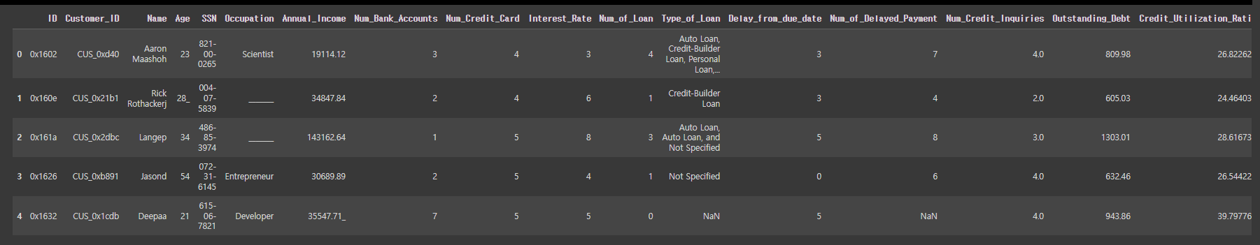
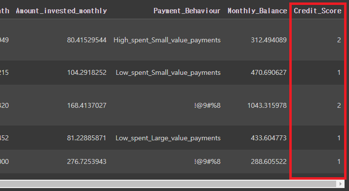
credit_df
(Credit_Score를 독립변수로 사용할 예정. 전처리할 부분이 많은 까다로운 데이터셋임을 참고하자.)
# df의 열을 모두 펼치기
pd.set_option('display.max_columns', 50)
credit_df.head()
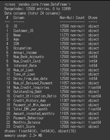
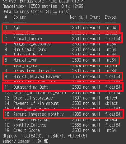
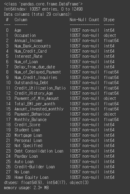
# info 확인
credit_df.info()
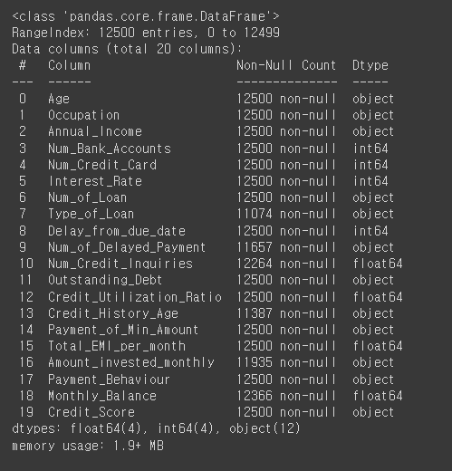
# 필요없는 열을 모두 찾아서 삭제
credit_df.drop(['ID', 'Customer_ID', 'Name', 'SSN'], axis=1, inplace=True)
credit_df.info()
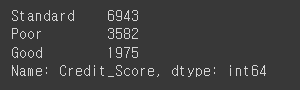
# credit_score의 value_counts 확인
credit_df['Credit_Score'].value_counts()
# credit_score를 숫자로 인코딩
credit_df['Credit_Score']=credit_df['Credit_Score'].replace({'Poor':0, 'Standard':1, 'Good':2})
credit_df.head()
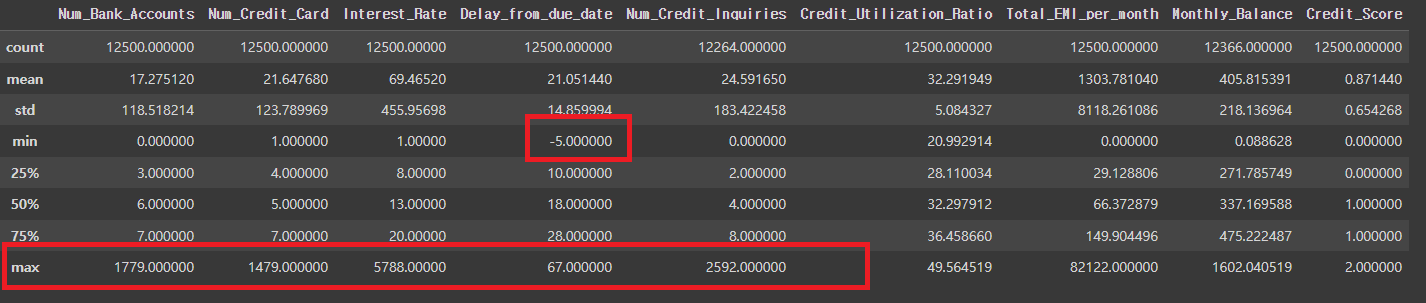
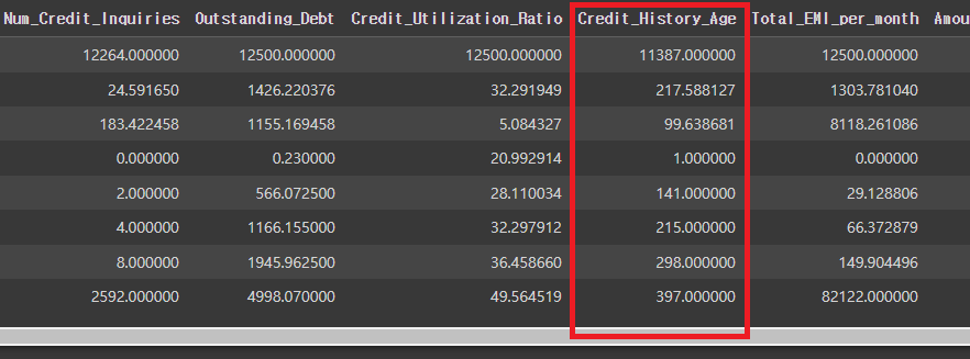
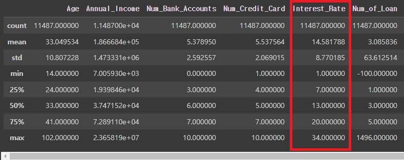
credit_df.describe()
# Num_Bank_Accounts, Num_Credit_Card 등의 max치가 이상치인 것으로 추정됨.
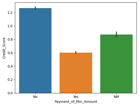
# 리볼빙과 신용점수의 관계에 대한 막대그래프
sns.barplot(x='Payment_of_Min_Amount', y='Credit_Score', data=credit_df)
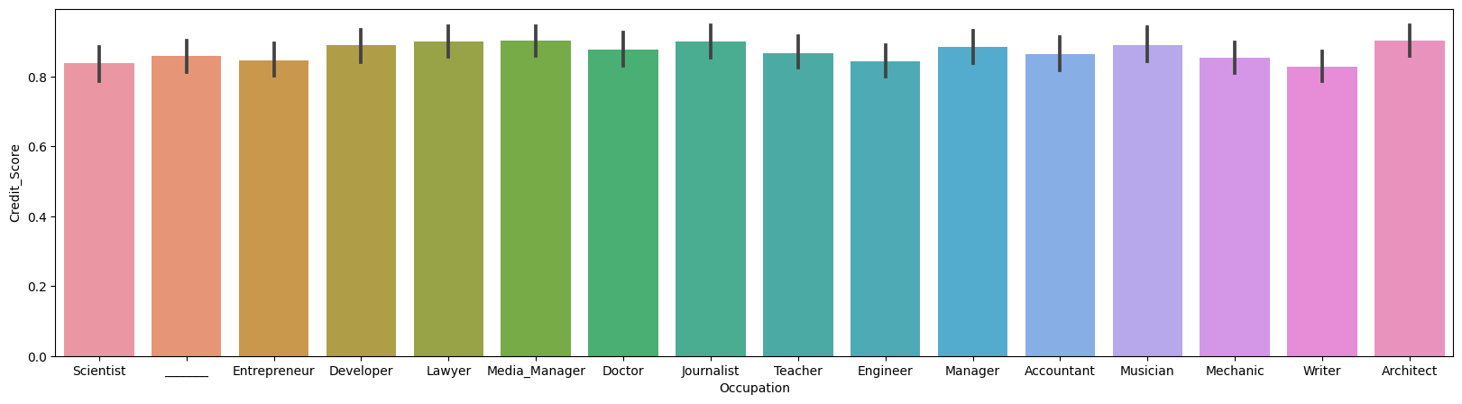
# 직업과 신용점수의 관계에 대한 막대그래프
plt.figure(figsize=(20,5))
sns.barplot(x='Occupation', y='Credit_Score', data=credit_df)
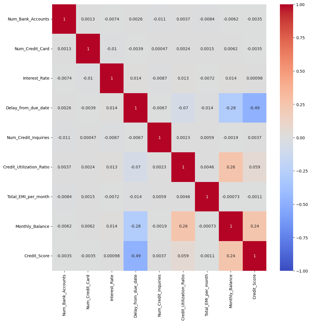
# 각 필드값에 대한 히트맵
plt.figure(figsize=(12,12)) # corr(): 각 열 간의 상관 계수를 반환
sns.heatmap(credit_df.corr(), cmap='coolwarm', vmin=-1, vmax=1, annot=True)
credit_df.info()

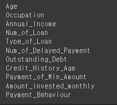
# object 인코딩
# 먼저 dtype이 O인 것들만 뽑음.
for i in credit_df.columns:
if credit_df[i].dtype == 'O':
print(i)
# Age, Annual_Income, Num_of_Loan, Num_of_Delayed_Payment, Outstanding_Debt, Amount_Invested_monthly 등의 수치들을 숫자로 변경
for i in ['Age', 'Annual_Income', 'Num_of_Loan', 'Num_of_Delayed_Payment', 'Outstanding_Debt', 'Amount_invested_monthly']:
credit_df[i] = pd.to_numeric(credit_df[i].str.replace('_','')) # 언더바(_)를 공백으로 변경
credit_df.info()
# 수치가 있는 object들이 int로 변경된 것을 볼 수 있음.
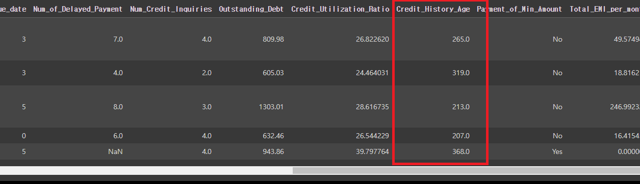
# Credit_History_Age(카드 사용기간)의 data를 개월로 변경
[ 예) 22 Years and 1 Months -> 22*12 + 1 ]
credit_df['Credit_History_Age'] = credit_df['Credit_History_Age'].str.replace(' Months', '')
credit_df['Credit_History_Age'] = pd.to_numeric(credit_df['Credit_History_Age'].str.split(' Years and ', expand=True)[0])*12 + pd.to_numeric(credit_df['Credit_History_Age'].str.split(' Years and ', expand=True)[1])
# expand=True: array가 아닌, dataframe으로 변경해줌.
credit_df.head()
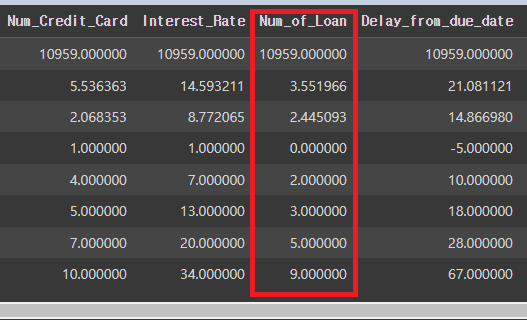
credit_df.describe()
# 이상치 (Age가 0보다 작은사람) 뽑아냄.
credit_df[credit_df['Age']<0]
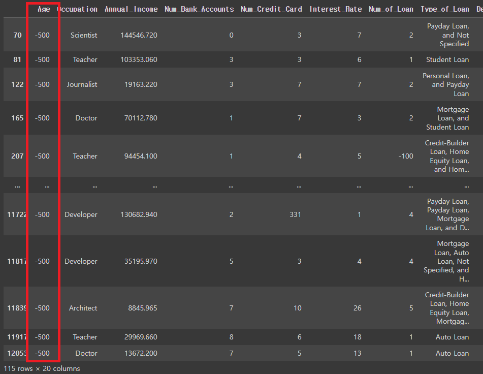
#Age가 0보다 큰 사람만 다시 데이터에 넣기
credit_df = credit_df[credit_df['Age']>=0]
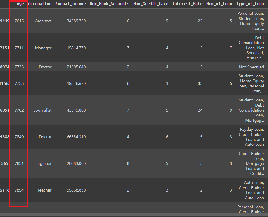
# Age가 비정상적으로 많은 경우 확인
credit_df.sort_values('Age').tail(30)
# Age에 대한 boxplot 확인
sns.boxplot(y=credit_df['Age'])
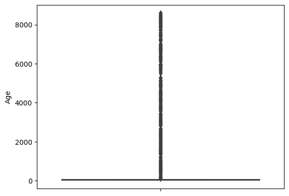
# 나이가 100살보다 큰 사람을 찾기 # 임의로 나이를 120살 아래까지 지정해주고 나머지는 거름.
credit_df[credit_df['Age']>100].sort_values('Age')
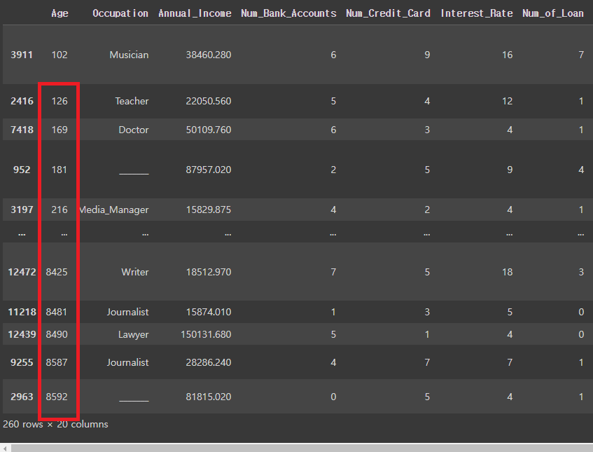
credit_df = credit_df[credit_df['Age']<120]
credit_df.describe()
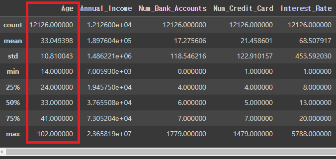
# Num_Bank_Accounts가 비정상적으로 많은 경우 확인
len(credit_df[credit_df['Num_Bank_Accounts']>10]) / len(credit_df)
# 수정
credit_df = credit_df[credit_df['Num_Bank_Accounts']<=10]
credit_df.describe()
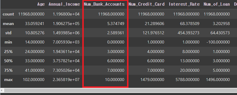
# Num_Credit_Card 비정상적으로 많은 경우 확인 후 수정
credit_df = credit_df[credit_df['Num_Credit_Card']<=10] # 10은 임의의 수
credit_df.describe()

# Interest_Rate 비정상적으로 많은 경우 확인 후 수정
credit_df = credit_df[credit_df['Interest_Rate']<=40] # 40은 임의의 수
credit_df.describe()
# Num_of_Loan 비정상적으로 많은 경우 확인 후 수정
credit_df = credit_df[(credit_df['Num_of_Loan']<=10) & (credit_df['Num_of_Loan']>=0)]
# 0이상 10이하는 임의의 범위
credit_df.describe()
# Num_of_Delayed_Payment 비정상적으로 많은 경우 확인 후 수정
credit_df = credit_df[(credit_df['Num_of_Delayed_Payment']<=30) & (credit_df['Num_of_Delayed_Payment']>=0)] # 0이상 30이하는 임의의 범위
# Num_Credit_Inquiries 비정상적으로 많은 경우 확인 후 수정
credit_df['Num_Credit_Inquiries'] = credit_df['Num_Credit_Inquiries'].fillna(0) # 결측치 0으로 대체
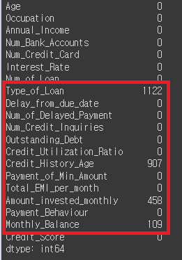
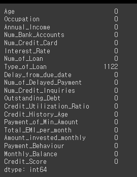
# 공백값의 총 갯수 확인
credit_df.isna().sum()
# Credit_History_Age, Amount_invested_monthly, Monthly_Balance을 모두 0으로 줄 예정
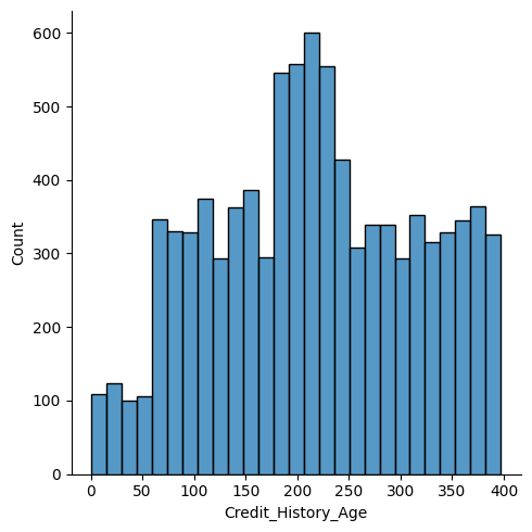
# Credit_History_Age의 displot 확인
sns.displot(credit_df['Credit_History_Age'])
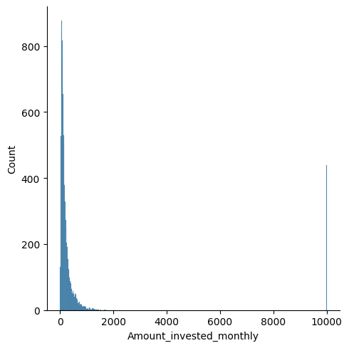
# Amount_invested_monthly displot 확인
sns.displot(credit_df['Amount_invested_monthly'])
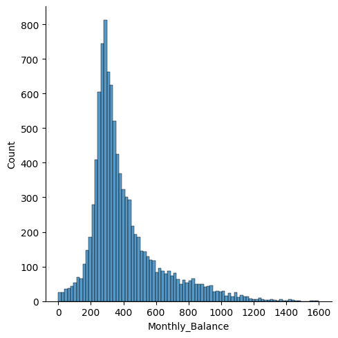
# Monthly_Balance displot 확인
sns.displot(credit_df['Monthly_Balance'])
# 결측값을 중간값으로 채운 경우
credit_df = credit_df.fillna(credit_df.median())
# 결측값의 총 갯수 확인
credit_df.isna().sum()
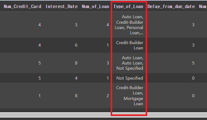
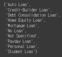
# 'Type_of_Loan'에 존재하는 모든 대출이름을 확인 후 'type_list'에 저장
credit_df['Type_of_Loan'] = credit_df['Type_of_Loan'].str.replace('and ','')
credit_df.head()
# NaN값을 No Loan으로 변경
credit_df['Type_of_Loan'] = credit_df['Type_of_Loan'].fillna('No Loan')
# type_list 확인
type_list = set(credit_df['Type_of_Loan'].str.split(', ').sum())
type_list
# lambda함수를 이용한 파생변수의 생성
for i in type_list:
credit_df[i] = credit_df['Type_of_Loan'].apply(lambda x: 1 if i in x else 0)
credit_df.head()

# 파생변수의 새로운 생성에 따라 필요없어진 Type_of_Loan 필드값 삭제
credit_df.drop('Type_of_Loan', axis=1, inplace=True)
credit_df.info()
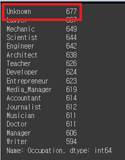
# Occupation의 value값 확인.
credit_df['Occupation'].value_counts()

# _______를 Unknown으로 변경
credit_df['Occupation'] = credit_df['Occupation'].replace('_______', 'Unknown')
# 확인
credit_df['Occupation'].value_counts()
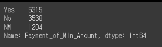
# Payment_of_Min_Amount의 value값 찾기
credit_df['Payment_of_Min_Amount'].value_counts()
# Payment_Behaviour value값 찾기
credit_df['Payment_Behaviour'].value_counts()
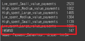
# !@9#%8 값 Unknown 변경 예정
credit_df['Payment_Behaviour'] = credit_df['Payment_Behaviour'].replace('!@9#%8', 'Unknown')
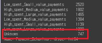
# 변경 확인
credit_df['Payment_Behaviour'].value_counts()
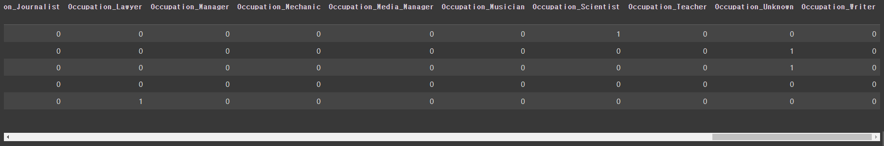
# 전처리작업 마무리
# Occupation, Payment_of_Min_Amount, Payment_Behaviour 모두 원핫인코딩
credit_df = pd.get_dummies(credit_df, columns={'Occupation', 'Payment_of_Min_Amount', 'Payment_Behaviour'})
# 변경 확인
credit_df.head()
# 데이터 분할
from sklearn.model_selection import train_test_split
# 데이터 갯수 확인
len(credit_df)

X_train, X_test, y_train, y_test = train_test_split(credit_df.drop('Credit_Score', axis=1), credit_df['Credit_Score'], test_size=0.2, random_state=10)
10-2. LightGBM(LGBM)
LightGBM은 Microsoft에서 개발한 오픈 소스 프로젝트로, 기존의 GBM(Gradient Boosting Machine)
알고리즘에 비해 더 빠른 학습 속도와 더 높은 성능을 제공하는
분산 학습 기반의 경량화된 기계 학습 알고리즘이다.
LightGBM은 데이터의 특성에 따라 성능을 향상시키는 효율적인 기능을 가지고 있다.
대용량 데이터셋에서도 높은 처리 속도를 유지하면서 정확도를 높일 수 있어,
대규모 데이터를 다루는 상황에서 많이 사용된다. (적은 데이터로 다룰 시, 과적합의 가능성이 높음)
LightGBM의 핵심 아이디어는 기존의 GBM 알고리즘에서 사용되는 트리 분할 방법을 개선한 것이다.
일반적으로 GBM은 균형 트리 분할 방법을 사용하는데, LightGBM은 leaf-wise 트리 분할 방법을 사용하여
보다 효율적인 분할을 수행한다. 이러한 분할 방법은 균형 트리 분할에 비해 더 적은 메모리를 사용하고,
더 빠른 학습 속도와 더 높은 정확도를 제공한다.
LightGBM은 다양한 응용 분야에서 사용될 수 있으며, 주로 분류(Classification)와 회귀(Regression) 문제에 적용된다. 또한, 특징 선택(Feature Selection), 이상 탐지(Anomaly Detection), 순위 학습(Ranking), 추천 시스템(Recommendation Systems) 등에도 사용될 수 있다.
# 사이킷런에서 지원하지 않음.
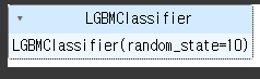
from lightgbm import LGBMClassifier
base_model = LGBMClassifier(random_state=10)
# 시험
base_model.fit(X_train, y_train)
# 예측
pred1 = base_model.predict(X_test)
from sklearn.metrics import accuracy_score, confusion_matrix, classification_report, roc_auc_score
# 정확도, 혼돈행렬, precision, recall, f1 score등의 리포트, 넓이에 대한 값 추출 등의 기능을 import
# 정확도
accuracy_score(y_test, pred1)

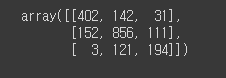
# 혼돈행렬
confusion_matrix(y_test, pred1)
# 어느정도 분포가 이루어진 것을 확인할 수 있음.
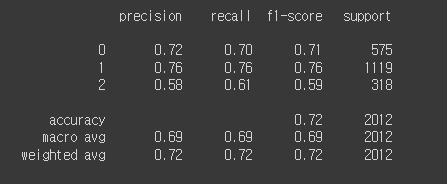
# report
확인
print(classification_report(y_test, pred1))
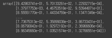
# proba 확인
proba1 = base_model.predict_proba(X_test)
proba1
# roc_auc_score 확인
roc_auc_score(y_test, proba1, multi_class='ovr')
# 'ovr'로 설정하면 "One-vs-Rest" 전략을 사용하여 다중 클래스 문제를 해결.
이 전략은 각 클래스를 기준으로 나머지 클래스들과 비교하여 이진 분류 문제로 변환하는 방법.
# 0.8896714282753299의 면적을 가짐
10-3. RandomizedSearchCV
scikit-learn 라이브러리에서 제공하는 하이퍼파라미터 튜닝 도구.
머신러닝 알고리즘에서 하이퍼파라미터는 모델의 학습과정을 제어하고 모델의 성능을 개선하는 데 사용되는 매개변수이다. 예를 들어, 결정 트리 알고리즘에서는 트리의 깊이, 분할 기준 등이 하이퍼파라미터에 해당함.
하이퍼파라미터의 선택은 모델의 성능에 큰 영향을 미칠 수 있으며,
이를 튜닝하여 최적의 조합을 찾는 것이 중요함.
RandomizedSearchCV는 하이퍼파라미터 튜닝을 위한 교차 검증을 수행함.
이를 통해 주어진 하이퍼파라미터 공간에서 랜덤하게 조합을 선택하여 모델을 학습하고 검증하는 과정을
반복하여 주어진 시간 및 횟수 안에서 최적의 하이퍼파라미터 조합을 찾음.
n_estimators: 반복수행하는 트리의 갯수(기본값: 100).
# 값을 크게 지정하면 학습시간도 오래걸리며, 과적합이 발생할 수 있음.
max_depth: 트리의 최대 깊이. (기본값: -1)
num_leaves: 남아있는 데이터.
learning_rate: 학습률(기본값:0.1)
# 파라미터 생성
params = {
'n_estimators':[100,300,500,1000],
'max_depth':[-1,30,50,100],
'num_leaves':[5,10,20,50],
'learning_rate':[0.01,0.05,0.1,0.5]
}
# lgbm 객체 생성
lgbm = LGBMClassifier(random_state=10)
# RandomizedSearchCV의 import
from sklearn.model_selection import RandomizedSearchCV
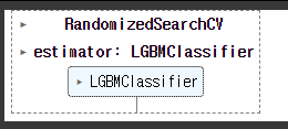
rand_lgbm = RandomizedSearchCV(lgbm, params, n_iter=30, random_state=10)
rand_lgbm.fit(X_train, y_train)
# 결과에 대한 report 출력
rand_lgbm.cv_results_

# 결과에 대한 최고의 params 출력
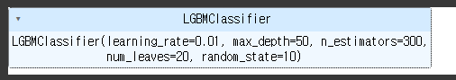
rand_lgbm.best_params_

lgbm = LGBMClassifier(random_state=10, num_leaves=20,n_estimators=300, max_depth=50, learning_rate=0.01)
# 교육
lgbm.fit(X_train, y_train)
# 예측 시험
proba = lgbm.predict_proba(X_test)
roc_auc_score(y_test, proba, multi_class='ovr')
# 하이퍼 파라미터 튜닝 전: 0.8896714282753299
# 하이퍼 파라미터 튜닝 후: 0.8978937021863681
# 튜닝 전후의 정확도 차이
0.8978937021863681-0.8896714282753299
하이퍼파라미터 값을 None으로 주는 것: 해당 하이퍼파라미터에 대한 기본값을 사용한다는 의미.
일반적으로 하이퍼파라미터에는 기본값이 미리 정해져 있으며, 이 값을 사용하고자 할 때 None을 할당함.


